StarFast - A Fast Simulation Tool for Testing Algorithms
Overview
StarFast is a simple but fast simulation tool to generate images for testing algorithms, and may be obtained from https://github.com/lsst-dm/starfast_simulator . It has been developed primarily with an aim to quickly generate many images affected by realistic Differential Chromatic Refraction (DCR) and astrometric errors, but it is hopefully general enough to be used for other cases when we need to test algorithms against simulated data.
It will generate a simulated catalog of stars (see Simulated catalogs below) and compute the flux in Janskys for each source given the instrument bandpass. For wavelength-dependent effects such as DCR, each band is divided into multiple sub-band planes. Sources are convolved with the PSF in Fourier space (but see Implementation below for details), and any sub-band planes are stacked to produce the final image. Noise may optionally be injected at any step, to simulate photon shot noise of the sources, flat spectrum sky noise, or noise from the electronics.
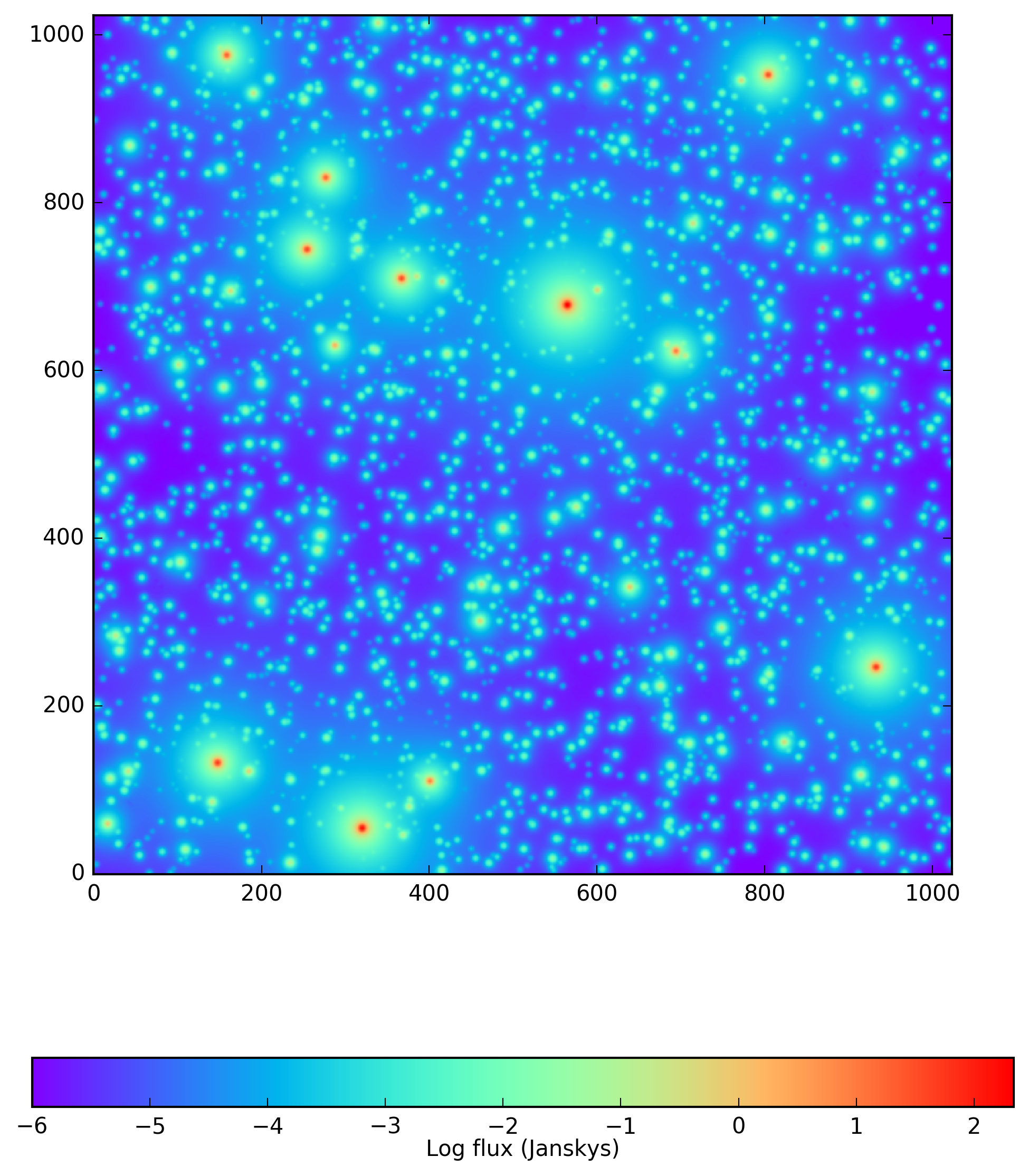
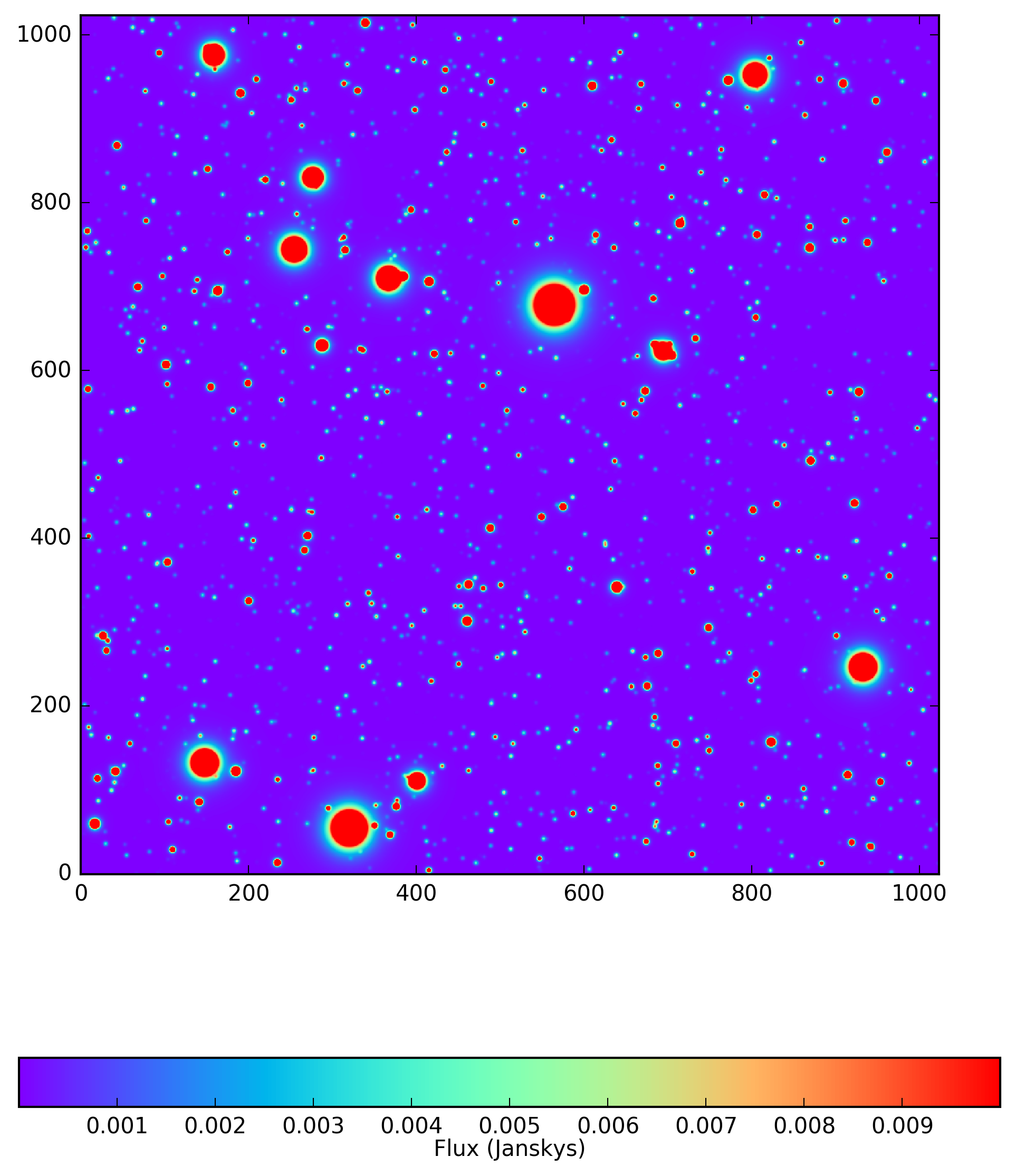
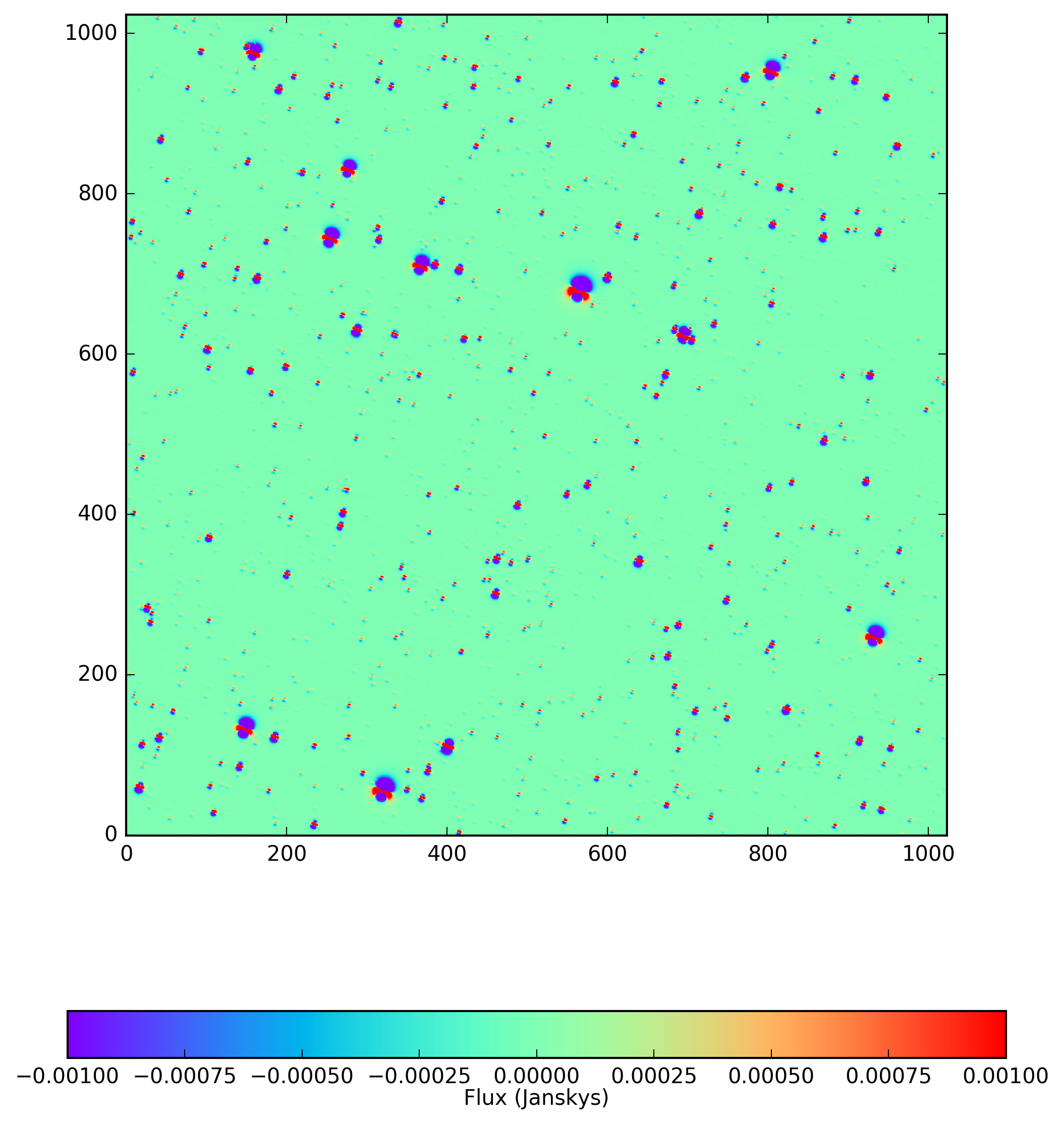
Several example images are shown below, which were produced using the included iPython notebook (https://github.com/lsst-dm/starfast_simulator/blob/master/StarFast_example.ipynb). Each image uses the same catalog of 10,000 stars, consisting of 5124 K, 3303 G, 1255 F, 274 A, and 44 B type stars (which can be obtained with the example notebook by setting seed = 5). For this simulation I have generated two LSST u-band images: a ‘reference’ image at an airmass of 1.00 near zenith that used a single plane, and a ‘science’ image at an airmass of 1.20 that used 24 planes (a wavelength resolution of 3nm). Each star in the simulation uses a simulated Kurucz SED from sims_photUtils (https://github.com/lsst/sims_photUtils), and a Kolmogorov PSF from Galsim (https://github.com/GalSim-developers/GalSim). The initial simulation took ~40s on a single core of a 2015 MacBook Pro, and the science and reference images in Figures 1-3 each took an additional 30s to generate. Further images of the same field in the same band would also take 30s on this machine, regardless of the number of sources in the field or the observing conditions (noise, elevation, or azimuth angle). New simulations of the same field but under substantially diferent conditions such as sky rotation angle or filter The science image is not visually different from the reference image on either color scale so only the difference image is displayed in Figure 3. Note that the very hot and bright B type stars have a DCR dipole in the opposite direction of the cooler stars, which is precisely what a DCR algorithm must be designed to correct.
Simulated catalogs
StarFast begins by creating a simulated catalog of stars with properties drawn from random distributions for the stellar types O-M in proportion to their local abundance. Simulated properties include temperature (in degrees K), luminosity (relative to solar), surface gravity (relative to solar), and metallicity (log, relative to solar). These properties are matched to Kurucz model SEDs from GalSim, which are scaled by the luminosity of each star and attenuated by distance and the instrument bandpass throughput to yield fluxes in Janskys. Alternately, a simple blackbody radiation spectrum (with the bandpass) can be used.
Each star is randomly placed within a simulated volume of observable space (a 1000ly cone) from which pixel coordinates and attenuation from distance are calculated, though no attempt is made to simulate realistic clustering. All of the random distributions, including stellar properties and coordinates, can be initialized from a user-supplied random number generator seed value, which allows for repeated simulations of the same patch of sky in different wavelength bands or to reproduce previous results. Simulated catalogs may also be returned and saved, so they may be modified by external tools if desired, and those saved catalogs may be supplied in place of generating a new random catalog from a seed.
Implementation
For those who don’t care for the gory details, StarFast uses a variant of standard FFT convolution with a PSF to simulate images. It plays a few tricks, however, to gain speed and avoid the common aliasing and ringing artifacts common to FFTs.
In particular, the simulated catalogs are gridded without performing a convolution with a PSF in the first step. Instead, for each pixel in the image plane, the 2D sinc function is computed for each star at its floating-point position, which gives the identical result as taking the direct Fourier transform of a delta function (not centered on a pixel) followed by an FFT back to the image plane, but without folding. If multiple images have a star at precisely the same location but with different amplitudes, which these “image-space Fourier components” can be re-used with a simple scaling. Additionally, because the function falls off as 1 / x * y off the column and row of pixels that the star lands in, it’s value quickly becomes insignificant. This means that, for faint stars, we only need to evaluate the function for a small percentage of the total image pixels: for a slice in x over all y, a slice in y for all x, and a small radius of pixels centered on the star. A Hanning window function is applied to the pixels included by radius that are not in the x or y slices, which suppresses ringing from the radial cut. Finally, very bright stars are evaluated separately using all pixels, and at twice the resolution to eliminate FFT artifacts.
To properly treat effects that vary over the bandwidth of a filter, StarFast constructs many planes for each image, each with a restricted wavelength range, and the SED of each star is integrated over the filter for the restricted wavelength range to produce a vector of fluxes. These sub-band flux values could each be gridded and convolved with the PSF separately, with the final images simply stacked to produce one image encompassing the full bandwidth, but this is very inefficient. Instead, StarFast generates the image-space Fourier components described above for each star, and scales the values by the sub-band amplitude for each plane. Each plane gets it’s own PSF model, and if there is a wavelength dependant position shift (such as with DCR), that is included in the PSF. Finally, the images are convolved with their PSFs using FFTs, and stacked.


